n-dodecane, 15 O2, 1000 K, 22.8 kg/m3
See Skeen et al. 2016 , Manin et al. 2013, and the ECN soot diagnostics page for the experimental methodology.
High-speed line-of-sight extinction imaging provides a time-resolved measure of the optical thickness (KL) throughout at large region of the spray flame as shown in the movie below.
| Download KL movie |
High-speed KL images are processed to determine the onset time of soot. The total mass within the entire spray flame at each time step is computed. The time at which the total mass of soot within the flame exceeds 0.5 µg defines the onset based on the total mass. The total soot mass as a function of time is shown below.

| Total soot mass (µg) as a function of time (ms) (right-click and select “save link as…”) |
High-speed KL images are also processed to determine the onset location and timing of soot based on the soot mass observed at each axial position. A threshold of 10 ng resulted in consistency between this method and the total mass technique shown above. An example of the spatially resolved soot mass as a function of time is shown in the movie below. The derived onset times and location are tabulated below
| Download soot mass movie (right-click and select “save link as…”) |
| Soot Onset Data | ||||||||
| Tambient | ρambient | O2,ambient | Fuel | Inj. Duration | Nozzle | tonset, total | tonset, axial | Onset location |
| [K] | kg/m3 | % | — | [ms] | — | [ms] | [ms] | [mm] |
| 1000 | 22.8 | 15 | DN | >4 | 370 | 0.47 | 0.49 | 24.3 |
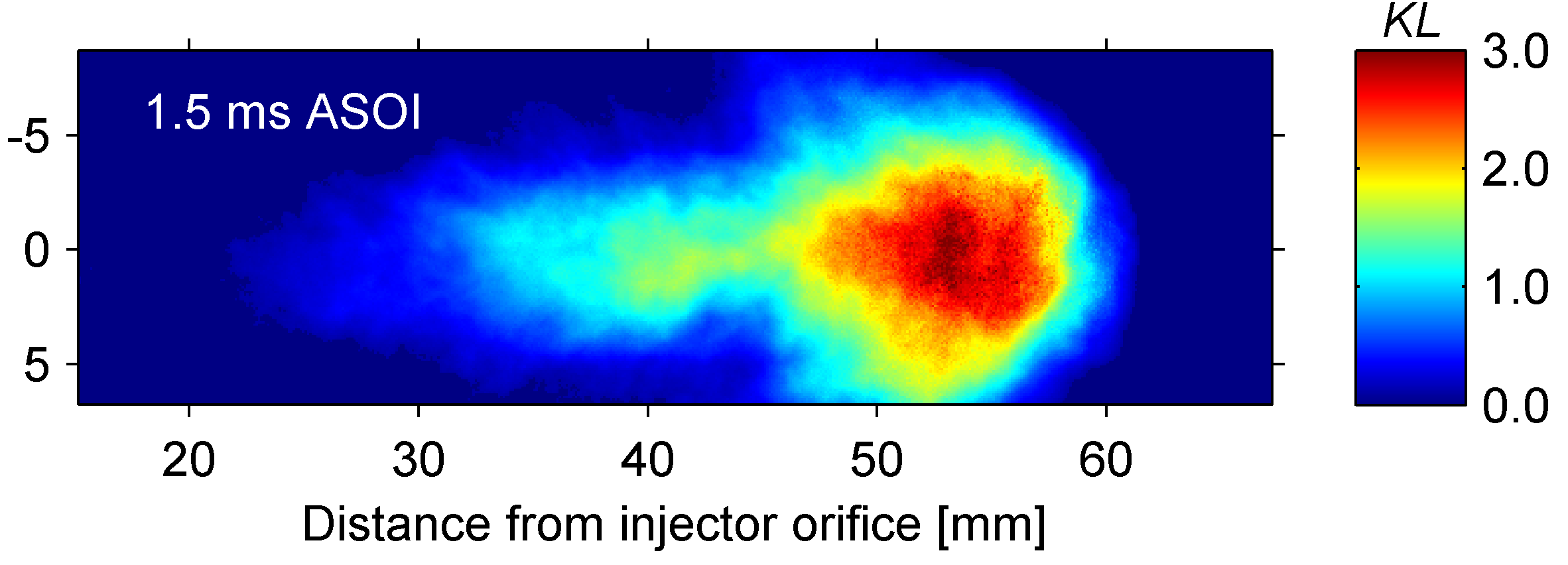
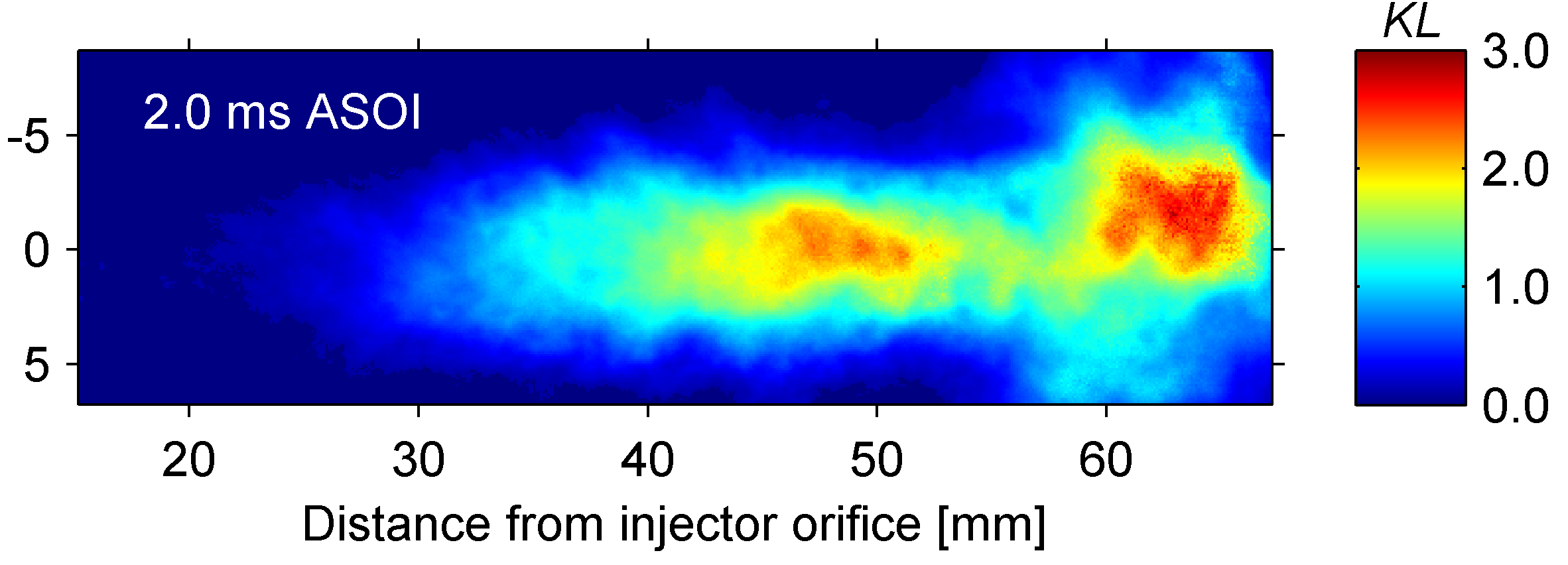
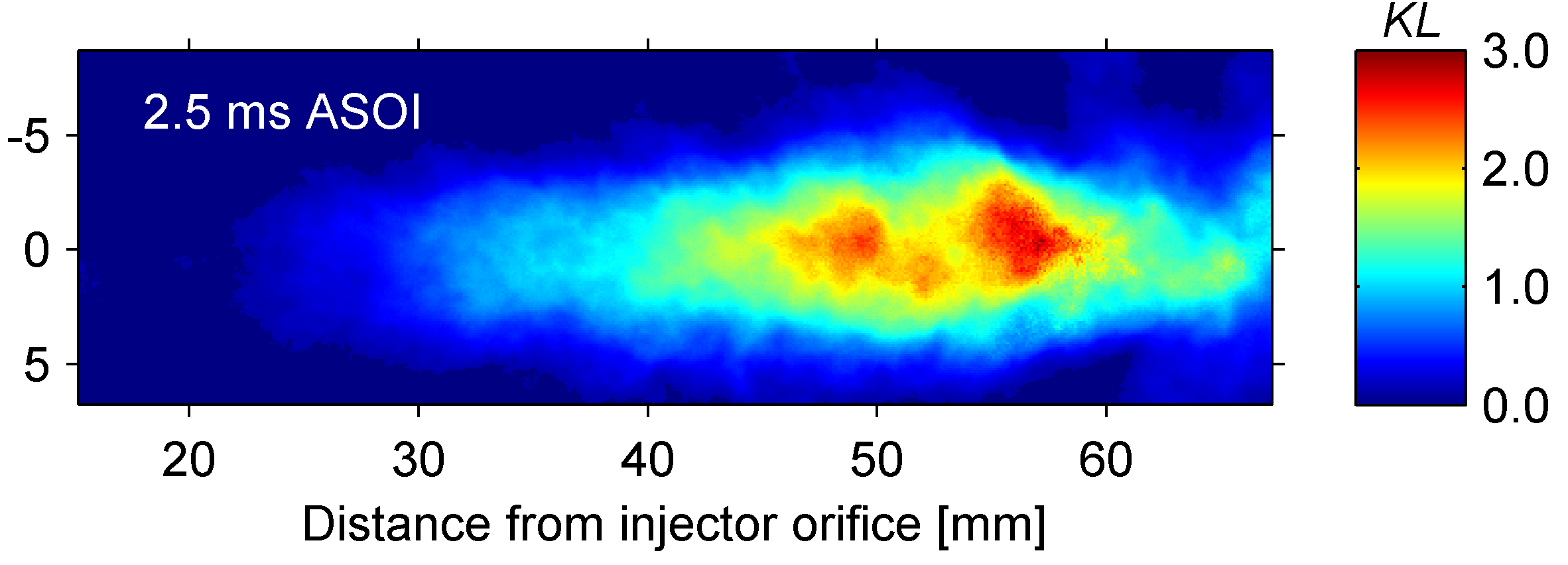
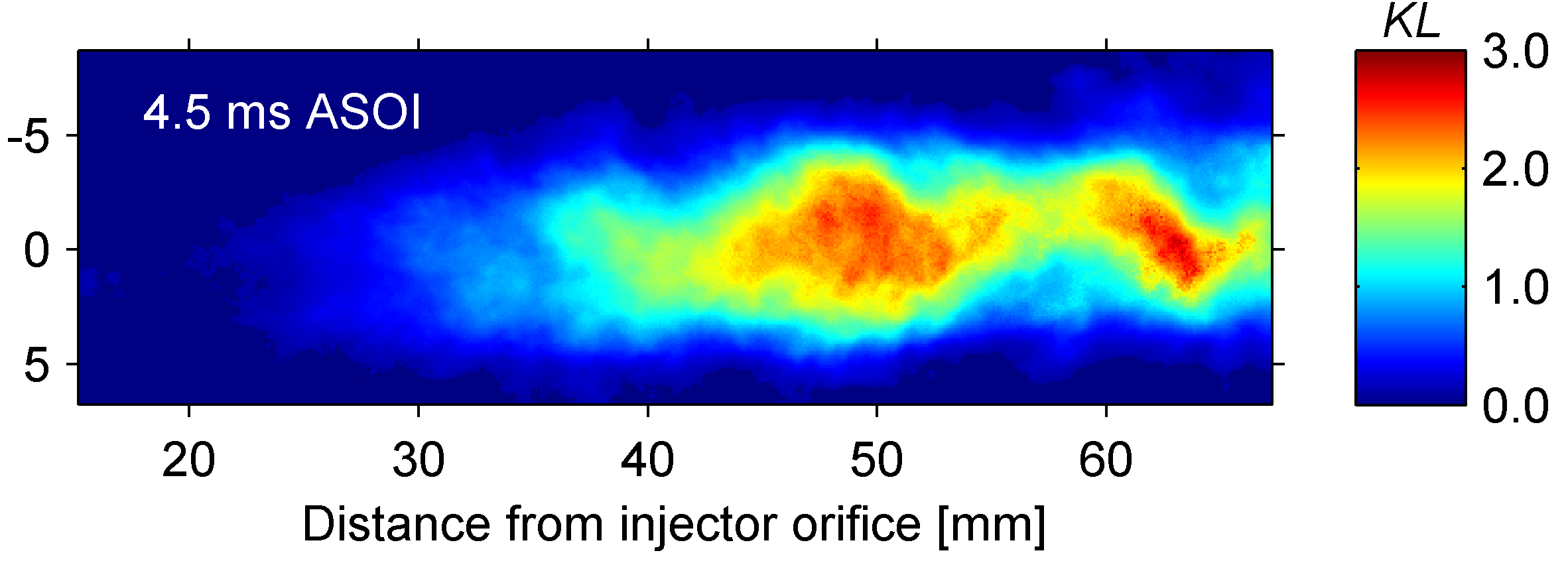
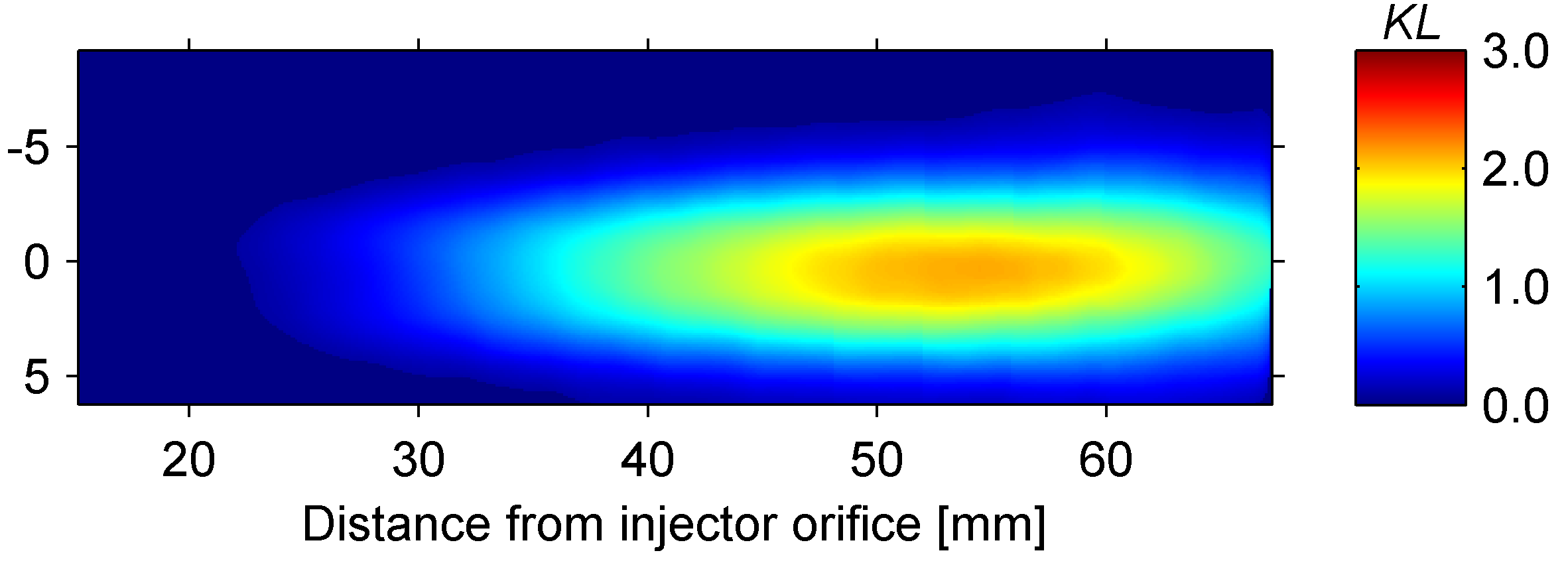
Optical Thickness, KL
The ensemble-averaged KL maps at 1.5 ms, 2.0 ms, 2.5 ms, and 4.5 ms ASOI are shown below. These images, in conjunction with the total soot mass at their respective timings from above, can be used as a target for modeling efforts of soot in the Spray A condition (and its parametric variants).
The time- and ensemble-averaged KL map during the quasi-steady period of a 6-ms injection is also provided below. The time-averaging was performed between 2.5 ms and 6 ms ASOI. The visible region of interest (ROI) in the experiment extends from 15.2 mm to 67.2 mm, thus model comparisons should be made only within this ROI.
| time ASOI [ms] | axial values (X) [mm] | radial values (Y) [mm] | 16-bit PNG | Scale for PNG+ | .csv |
| 1.5 | X | Y | KL 1.5 ms PNG | 2.0227e+04 | KL 1.5 ms CSV |
| time ASOI [ms] | axial values (X) [mm] | radial values (Y) [mm] | 16-bit PNG | Scale for PNG+ | .csv |
| 2.0 | X | Y | KL 2.0 ms PNG | 2.2599e+04 | KL 2.0 ms CSV |
| time ASOI [ms] | axial values (X) [mm] | radial values (Y) [mm] | 16-bit PNG | Scale for PNG+ | .csv |
| 2.5 | X | Y | KL 2.5 ms PNG | 2.2066e+04 | KL 2.5 ms CSV |
| time ASOI [ms] | axial values (X) [mm] | radial values (Y) [mm] | 16-bit PNG | Scale for PNG+ | .csv |
| 4.5 | X | Y | KL 4.5 ms PNG | 2.2141e+04 | KL 4.5 ms CSV |
| time ASOI [ms] | axial values (X) [mm] | radial values (Y) [mm] | 16-bit PNG | Scale for PNG+ | .csv |
| quasi-steady | X | Y | KL quasi-steady ms PNG | 3.0768e+04 | KL quasi-steady CSV |
| Soot Mass Data (DN, 1000 K, 22.8 kg/m3, 15% O2, Nozzle: 370, Inj. duration >4 ms) |
| time ASOI | masssoot |
[ms][μg]1.542.582.046.322.539.604.543.07quasi-steady41.80
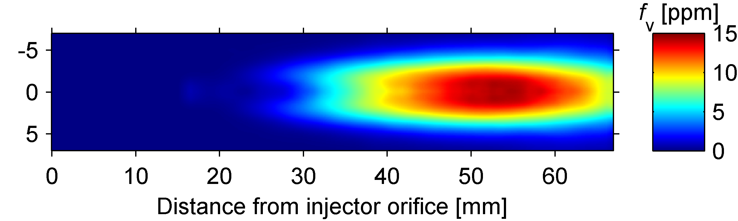
Soot Volume Fraction fv
Time-averaging over the quasi-steady period for each injection and subsequently ensemble-averaging multiple injection events yields an axisymmetric KL map that can be tomographically inverted to yield soot volume fraction, fv. For the fv map below, the incident LED light was centered at 406 nm and the non-dimensional extinction coefficient was determined to be 7.76 from Rayleigh-Debye-Gans theory for fractal aggregates. For more information see Manin et al. SAE-PFL-2013
| time ASOI [ms] | axial values (X) [mm] | radial values (Y) [mm] | 16-bit PNG | Scale for PNG+ | .csv |
| quasi-steady | X | Y | fv quasi-steady ms PNG | 4.5448e+03 | fv quasi-steady CSV |
Last updated 12 March 2014