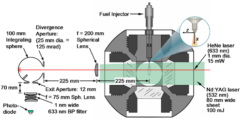
Fig. 4.5.1 Schematic of the combustion vessel and optical setup for soot measurements
Laser extinction and planar laser-induced incandescence (PLII) were used to make quantitative measurements of soot in a diesel jet. The setup is shown in Fig. 4.5.1 as reported in (Musculus, 2005). For laser extinction, a modulated (50kHz), 15-mW, 1-mm diameter HeNe laser beam (632.8 nm) was passed through sooting regions of a fuel jet and collected by an integrating sphere, narrow bandpass filter, and photodiode. This collection system accounts for beam-steering effects caused by refractive index gradients in the reacting jet and minimizes background interference from soot luminosity.
Transmitted laser intensities were related to soot optical thickness, KL, using the relationship:
![]()
where K is extinction coefficient, L is path length through the soot, and I and I 0 are transmitted laser intensities with and without soot present, respectively. The above intensities were corrected for background soot luminosity with the modulated laser turned off. The optical thickness can be quantitatively related to the soot volume fraction, fv(z) (volume of soot per unit volume), along the path of the laser using small particle Mie theory:
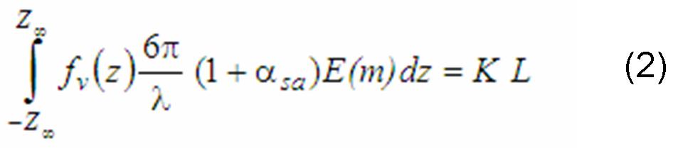
where Z∞ is the cross-stream position far outside of the jet, λ is the laser wavelength, αsa is the scattering-to-absorption ratio, E(m) = -Im[(m2-1)/(m2+2)], and m is the refractive index of soot. A value of (1+αsa)E(m) = 0.26 was used initially to relate the KL to soot volume fraction (Pickett, 2004). Note that while a quantitative relationship between KL and soot volume fraction is affected by uncertainties in the soot optical properties, a relative comparison between various operating conditions will be valid if the soot optical properties do not change significantly with changes in these conditions. At this point, we have no indication of a change in optical properties for carbon-dominant particles within high-temperature regions of the flame (Pickett, 2004). While still exhibiting significant uncertainty, later measurements have now suggested a values of (1+αsa)E(m) ≈ 0.46 for post-flame particulate from atmospheric burners (e.g. Zhu, 2002; Williams, 2007), which has been adopted for all ECN soot data. This change will make soot volume fractions reported in the database smaller, by a factor of 0.56.
PLII images were obtained by passing a thin (0.3 mm) Nd:YAG laser sheet (532 nm) through the fuel jet centerline as shown in Fig. 4.5.1. The PLII signal was imaged with an intensified CCD camera (50 ns gate). The lens and filters used were a Nikkor 105 mm, f/2.8 lens, a 450 nm short-pass filter, and a zero-incidence 532 nm laser mirror. Multiple PLII images were obtained for separate injection events at the same experimental conditions and timing.
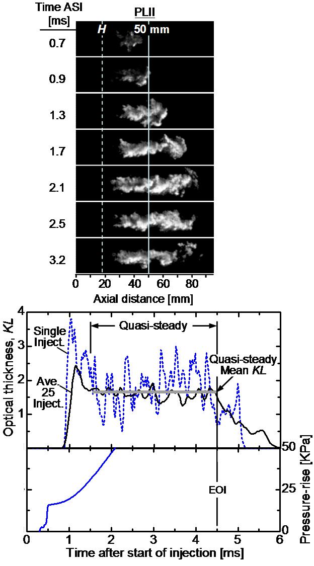
Fig. 4.5.2 Time-averaging of soot measurements.
Laser extinction measurements were time-averaged over the quasi-steady, mixing-controlled phase of the combustion event. Figure 4.5.2 illustrates the method. Figure 4.5.2 shows PLII images acquired at specific times after the start of injection (ASI) at the top and time-resolved KL profiles and the combustion vessel pressure-rise at the bottom. KL measurements are shown for a single injection event as a dashed line and for the average of 25 separate injection events as a solid line. The laser beam for the extinction measurement was positioned to pass through the centerline of the fuel jet at an axial position of x = 50 mm. For reference, both the x = 50 mm position (a solid vertical line) and the time-averaged, quasi-steady lift-off length (a dashed vertical line at 18.3 mm) are given on the PLII images.
The image sequence shows the jet progression from shortly after autoignition to well into the mixing-controlled combustion phase. For the conditions of Fig. 4.5.2, autoignition and the transient premixed burn begin at approximately 0.5 ms ASI as indicated by the sudden increase in pressure-rise. The PLII images show that soot begins to form shortly after autoignition at 0.7 ms ASI. At 0.9 ms ASI, the jet head reaches x = 50 mm and there is a rapid rise in KL. The PLII images indicate that the wider soot region at the penetrating tip of the jet passes through the x = 50 mm location between 0.9-1.3 ms ASI. After approximately 1.3 ms ASI, the images indicate that there are variations in soot level and width of the sooting region of the fuel jet at x = 50 mm, but that there is little change in general features of the jet with increasing time.
The time-resolved KL profiles reflect the general trends shown in the image time-sequence. High values of KL that occur between 0.9-1.3 ms ASI reflect the longer soot path length and the substantial soot levels in the transient head of the fuel jet as it passes the extinction measurement location. However, after the head of the jet passes the extinction measurement location, the KL value drops and varies about a mean value (indicated by the horizontal line in the plot) until the end of injection at 4.5 ms ASI. While the head of the jet is transient and continues to penetrate across the combustion vessel, the establishment of a mean KL value between 1.5 – 4.5 ms ASI suggests that a quasi-steady condition is reached in the fuel jet after the transient head passes. Fluctuations in KL after the transient head passes are explained by variations in the soot concentration and the width of the sooting region observed in the PLII images at the measurement location.
The quasi-steady nature of the fuel jet was utilized in reducing the soot data. KL values were time-averaged over the
quasi-steady portion of the injection event at any measurement location (i.e. the time between the head of the jet passing and the EOI). This timing window was chosen appropriately depending on the ambient conditions and axial position. An example of the exact timings utilized and along with downloadable, time-resolved KL data is given. The quasi-steady character of the jet was also utilized in acquiring time-averaged OH chemiluminescence images. The quasi-steady lift-off length (H) shown in Fig. 4.5.2 was determined from time-averaged OH chemiluminescence imaging, also from 1.5 to 4.5 ms ASI.
Typically, 10-15 separate simulations and injections were performed at each laser position to obtain statistical convergence of the average KL. For this number of injections, the mean KL value (Eq. (2)) has a 95% confidence interval(based on ±2σ/Ns0.5 where σ is the standard deviation and Ns is the number of samples) of approximately ±4% (Pickett, 2004).
A composite-average of the PLII images taken during quasi-steady combustion was used in combination with KL measurements at the jet centerline to obtain the time-averaged radial soot volume fraction profile (Idicheria, 2005). Since the PLII signal is proportional to the soot volume fraction (i.e., fv = C·LII), Eq. (2) shows that the measured LII profile, measured KL, and known soot optical properties make it possible to determine the calibration constant C, and hence, the radial soot volume fraction distribution.
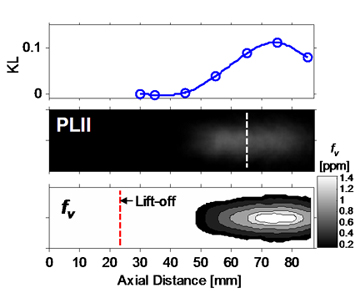
Fig. 4.5.3. Experimental method for determination of local soot volume fraction. (Top) Axial KL distribution. (Middle) Composite-average PLII. (Bottom) Soot volume fraction. Ambient conditions: Ta 1000 K, ρa 14.8 kg/m3, 15% O2. Injector conditions: 1500 bar above ambient, 0.1 mm nozzle, n-heptane
Figures 4.5.3 and 4.5.4 illustrate the technique described above. At the top and middle of Fig. 4.5.3 are the average KL and PLII, respectively, for a sample operating condition. The KL and PLII measurements show that soot begins to form at about 45 mm from the injector. The LII intensity distribution at 65 mm (dashed line) is given in Fig. 4.5.4. Using the measured KL and LII distribution at this position, a radial distribution of fv is obtained using Eq. (2) as shown at the right-hand axis of Fig. 4.5.4. The fv distribution was also forced to be axi-symmetric, as justified by the closeness of the fit to the original LII data. The technique was extended further to obtain the entire fv distribution of the jet by interpolating between KL measurements at many axial positions of the jet and using the LII information at the bottom of Fig. 4.5.3.
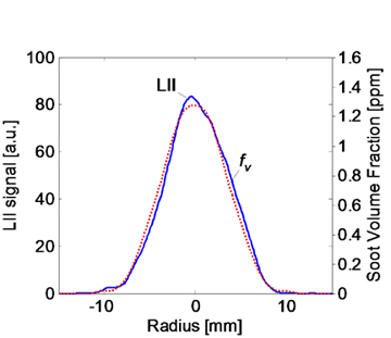
Fig. 4.5.4. LII and soot volume fraction radial profile at 65 mm from the injector for conditions of Fig. 4.5.2
The fv contour resembles the original PLII image intensity, but peak values are shifted downstream slightly. This is most likely caused by variation in the PLII laser sheet intensity. Other uncertainties affecting PLII measurement at diesel conditions are addressed in Pickett, 2006.
The KL measurement provides the calibration constant that corrects for these uncertainties along the axial length of the jet while the PLII measurement only provides information about the radial distribution of the soot.