See SAE 2007-01-0647 and SAE 2011-01-0686 for the experimental methodology.
Since the first release of this data, images have been reprocessed to consider uncertainties and the effect of spatial filtering via median filtering on the mean, standard deviation (or variance) and overall uncertainty. The table below lists the format of the newly processed images.
| pixels/mm | radial/axial pixels | radial values [mm] | axial values [mm] | median filter for mean | median filter for std. dev. |
| 20.90 | 600 x 826 | -14.2 to 14.4 | 16.4 to 55.8 | 13 x 13 pixels | 9 x 9 pixels |
Raw, instantaneous images are processed without applying any image filtering, but to remove particles and laser beam steering artifacts, additional spatial filtering is required on these images before computing statistics for the set of images. As shown in the figures below, spatial filtering does not significantly change the mean result (left), but larger median filters do decrease the apparent standard deviation (and uncertainty) as expected (right). At the same time, particles or laser artifacts, obviously are erroneous and increase the standard deviation. A suitable compromise is to use two sets of median filters. As shown in the table, a larger median filter (13×13 pixels) is applied to safely remove artifacts without changing the mean result. A smaller median filter (9×9 pixels) is applied to compute the standard deviation to prevent overfiltering, but particles and noise evidently remain in the standard deviation “image”. To remove these noise effects, while not reducing the standard deviation, a large (17×17 pixels) spatial filter is then applied. Note that the standard deviation results show (see figure) that the level is unchanged if a large filter is applied afterwards, but fluctuations are removed. To date, this last spatial filter is the best technique attempted to dynamically remove noise artifacts while not compromising (decreasing) the standard deviation. Also note that image spatial filtering is only one aspect of measurement resolution bias as a finite laser sheet thickness (approaching 0.5 mm with beam steering) also enlarges the spatial resolution.
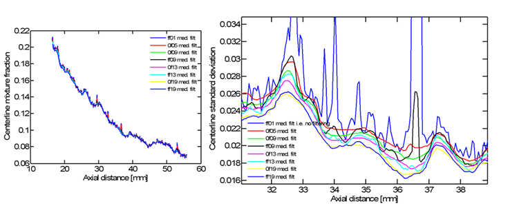
Fig. 1: Effect of median filtering on centerline statistics. Filter size for individual images is indicated in legend as ??xx where xx is the filter size. ffxx indicates no spatial filter is applied to the end result, while 0fxx indicates a final filter is applied.
Results
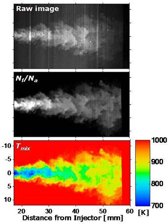
Ensemble-averaged data or instaneous images are stored as .png image files, but also as zipped text files, in terms of fuel mixture fraction (or fuel mass fraction as the system is inert with 0% ambient oxygen). Convert 16-bit png images to mixture fraction Z using Z=png*maxImg/(2^16), where maxImg is listed in the table below. Scale, axial, and radial dimensions are given above. The time after start of injection TASI for statistics is featured. Column 2 is mean mixture fraction. Column 3 is standard deviation, which is the square root of the variance. Standard deviation is given to ensure consistency in the units (all in terms of mixture fraction). Column 4 is mean mixture fraction uncertainty, computed using bias error uncertainty, the standard deviation and the number of samples. To express a 95% confidence interval in the mean, use mean value ± this uncertainty. Note that uncertaintes are relatively high because only 30-40 images are available at each time ASI (see SAE 2011-01-0686). Column 5 is standard deviation uncertainty computed using parameters similar to the mean. Column 6 is ensemble-averaged mean mixture temperature, computed using adiabatic mixing relationships for Spray H fuel and ambient conditions. Convert 16-bit png images to temperature T in [K] using T=png*450/(2^16) + 600 (i.e. the range of the images is 600 to 1050 K).
Instantaneous mixture fraction and temperature .png images are also available for download and analysis via these 43 MB zip files. All images were filtered with a 13×13 median filter. Convert 16-bit png images to mixture fraction Z using Z=png*0.35/(2^16) and temperature T in [K] using T=png*450/(2^16) + 600. The spatial scale and axial and radial range are the same as the average data provided.