Spray A Injector 210675
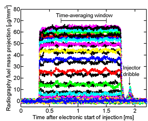
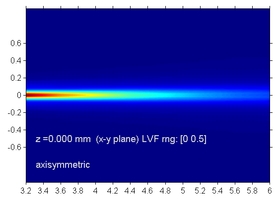
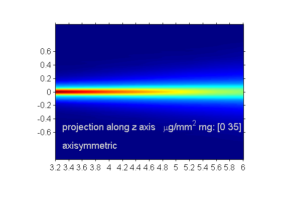
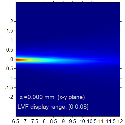
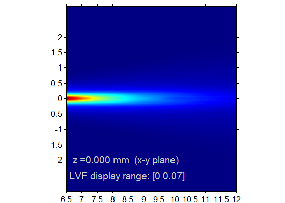
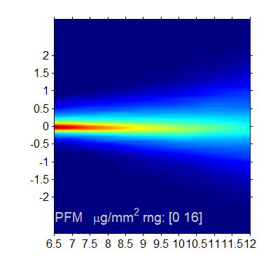
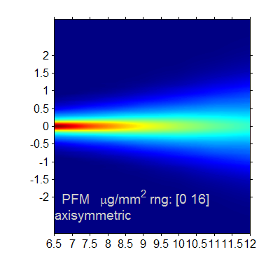
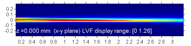
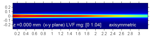
X-ray radiography of the projected fuel mass has been analyzed to derive the fuel mass density and liquid volume fraction in the near nozzle field at Spray A operating conditions, and 303 K ambient temperature. As detailed in Kastengren et al. (2012) and Pickett et al. (2014), a small (5-6 µm) x-ray beam is passed through the fuel spray to measure of the fuel mass along its beam path. A 2D raster scan is obtained with 4 different injector rotations. Time-resolved data from many injections are used to measure the fuel distribution with respect to time, as well as an average during the steady state, as shown in the figure (many radial positions at an axial position fixed at x = 0.1 mm). Tomography is performed to derive local (3D) quantities, rather than line-of-sight or “projection” data.
Tables below provide measured quantities at different positions, with reference to the Spray A nozzle geometry convention where x, y, and z are the axial, vertical, and horizontal coordinates, respectively. The local fuel concentration (density) from the tomographic reconstruction is converted to liquid volume fraction (LVF) by dividing a fuel density of 720 kg/m3 corresponding to the measured temperature of the nozzle of 333 K. Measurements are re-sampled by interpolation to provide intermediate x,y,z values as demonstrated in these rotating or “fly-through” movies.
“Steady-state” liquid volume fraction and z-axis fuel mass integral (projection):
a time average from 0.4 ms to 1.2 ms after actual start of injection.
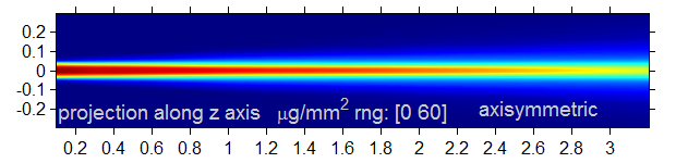
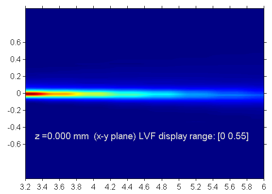
| Axial distances [mm] | y (column), z (rows), x (rows) | y-z LVF | x-y LVF | x-y LVF Axis-symmetric average | z-axis projected fuel mass | z-axis projected fuel mass, axis-symmetric |
| Range of axial distances for data package (e.g. zip file). Naming convention example: “s675x0.4”–> steady, nozzle serial, axial in mm. | Vectors giving the dimensions for the y (column), z(rows), or x(rows) corresponding to each pixel. Note that y is given in descending order corresponding to the ECN convention with the top of the displayed image as positive (i.e. first row of image/data is positive y). Likewise for z. | Liquid volume fraction in the y-z cut plane. Data stored in zip files with .csv datafiles or .png, usually in 0.1 mm axial intervals. See *g.png file for layout and max range LVF of png file. | Liquid volume fraction in the x-y cut plane. Measured .png and .csv data files. | Liquid volume fraction in the x-y cut plane. Processed with axis-symmetric averaging. | Integral of fuel mass (density) along z-axis, yielding an x-y “projection image” of µg/mm^2. See *g.png file for layout and max range of png file. | Integral of fuel mass (density) along z-axis axis-symmetric, yielding an x-y “projection image” of µg/mm^2 |
| 0.1 to 3.0 mm | -0.3:0.3 mm radial rng y(column) z(row) x(row) |
LVF .zip file | *g.png LVF png data .csv |
*g.png LVF png data .csv |
*g.png FPM png data .csv |
*g.png FPM png data .csv |
| 3.0 to 6.0 mm | -1.0:1.0 mm y(column) z(row) x(row) |
LVF .zip file | *g.png LVF png data .csv |
*g.png LVF png data .csv |
*g.png FPM png data .csv |
*g.png FPM png data .csv |
| 6.0 to 12.0 mm | -3.0:3.0 mm y(column) z(row) x(row) |
LVF .zip file | *g.png LVF png data .csv |
*g.png LVF png data .csv |
*g.png FPM png data .csv |
*g.png FPM png data .csv |
| Examples: | *g.png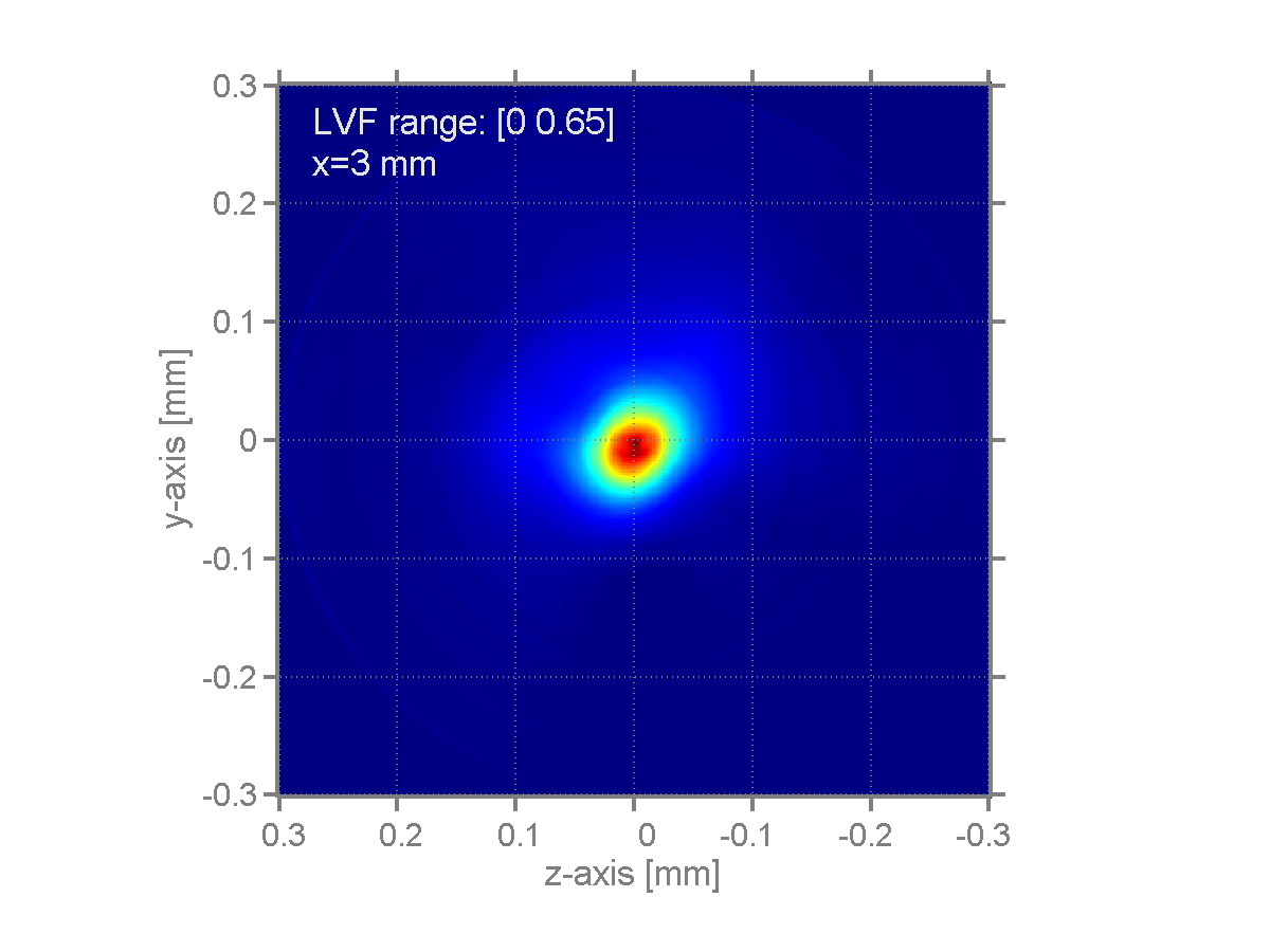 |
LVF png |
y-z data .csv file at x = 3 mm |
 |
 |
Transverse integrated mass (TIM) µg/mm vs axial distance [mm]. An integral of the fuel mass projection in the transverse (y or z) direction quantifies the fuel mass per unit axial distance. Download TIM vs x in two column data .csv file