Surrogate Fuel 77% dodecane and 23% m-xylene
See SAE 2005-01-3834 and the ECN soot diagnostics page for the experimental methodology.
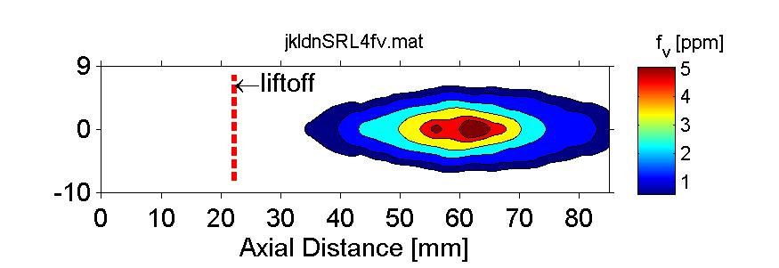
Line-of-sight extinction (KL) data are combined with soot profile LII imaging to generate quasi-steady soot volume fraction distributions as given below. The data is for the axis plane of the injector, beginning at the nozzle.
A vector graphics plot is available via the following link: view the vector graphics plot
| soot volume fraction 2D data in ppm |
| soot volume fraction 2D data as png image (200 x 640) |
| Data scale: 6.4 pix/mm | Nozzle origin: pixel 100,1 | Maximum FV: 0.7758 [ppm] | Convert png to soot volume fraction: scale the image by (Maximum FV)/255 |
 A vector graphics plot is available view svg
Soot volume fraction fv is obtained via KL = ∫ fv ke / λ dz where ke is the optical extinction coefficient, λ is wavelength (632.8 nm) and z is the direction of the laser path. The optical extinction coefficent used to convert the extinction data to soot volume fraction is ke = 8.7. There has been convergence towards this value in the literature (e.g. Zhu, 2002; Williams, 2007).
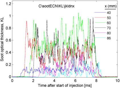
Ensemble-average KL data are available for comparison to modeling predictions in the table below. As shown at the right, the KL increases initially when the spray arrives at a particular location, or when soot formation begins after ignition (e.g. x = 40 mm data). The jet arrival, soot formation, and fluctuation are consistent with high speed soot luminosity imaging for this condition. Although fluctuations in KL are apparent in the figure, these data are actually the ensemble-average of typically 10 or more injections; the few number of injections means that the data are not completely converged to the actual ensemble mean. But there is evidence that fluctuations occur about a quasi-steady mean after the head of the jet passes and before the end of injection. Time-averaging windows were identified (see table) to give a time-averaged KL at a particular position (also given in table). These time-averaged KL were used to derive the soot volume fraction field given above.
| Axial position [mm] | Cross-stream position [mm] | Time-average start [ms] | Time-average end [ms] | Time-average KL | Ensemble-average KL with respect to time, including standard deviation and uncertainty |
| 40.0 | 0.0 | 3.0 | 7.0 | 0.114 | KLvsTime |
| 50.0 | 0.0 | 3.0 | 7.0 | 0.370 | KLvsTime |
| 60.0 | 0.0 | 3.0 | 7.0 | 0.609 | KLvsTime |
| 70.0 | 0.0 | 3.0 | 7.0 | 0.372 | KLvsTime |
| 80.0 | 0.0 | 3.0 | 7.0 | 0.147 | KLvsTime |
| 86.0 | 0.0 | 3.0 | 7.0 | 0.071 | KLvsTime |